Big Data on AWS Deep Dive (Part 8): Online Feature Stores — DynamoDB, ElastiCache, and OpenSearch k-NN

Why an Online Serving Layer?

A recommendation request must return within 200ms. You cannot query a data warehouse or data lake at that latency — you need a dedicated online serving layer.

This chapter explains four online storage systems — DynamoDB, ElastiCache (Redis), OpenSearch k-NN, and Neptune — what each is best at, and how to choose between them.

---

Overall Division of Responsibilities

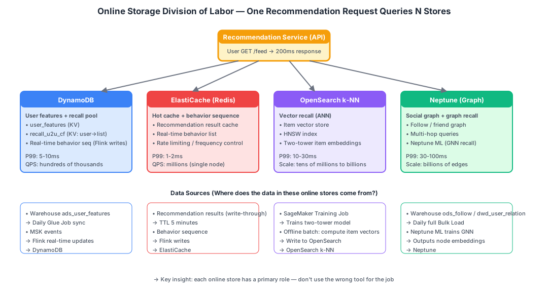
A single recommendation request (GET /feed?user_id=123) may query four different online stores:

Recommendation Service (200ms budget)
  │
  ├─[10ms]── DynamoDB    : Fetch user features + recall pool cache
  ├─[2ms]─── Redis       : Fetch real-time behavior sequence + last recommendation cache
  ├─[20ms]── OpenSearch k-NN: User vector → ANN find items
  └─[50ms]── Neptune     : Second-degree friends / graph recall (on demand)
  │
  ▼
SageMaker Endpoint (ranking model scoring, 30ms)
  │
  ▼
Return Top 10

Key insight: Each store has its “home turf” — avoid mixing responsibilities.

---

Amazon DynamoDB

What It Is

AWS’s managed KV / document database. Most important characteristics:

• Millisecond reads and writes (P99 under 10ms)
• Auto-scales to hundreds of thousands of QPS
• Fully serverless (billed by read/write units and storage)
• Schema-free (each row can have different fields)

Data Model

Table: user_features
  Partition Key: user_id (String)
  Sort Key: <optional>

Item:
{
  "user_id": "12345",
  "age": 25,
  "city": "Shanghai",
  "tags": ["food", "travel"],
  "last_5_clicks": ["v_001", "v_002", ...],
  "ctr_7d": 0.054,
  ...
}

Each row is called an Item, with a maximum size of 400 KB.

Pricing Model

Two capacity modes:

Mode	Billing	Best For
On-Demand	$0.25 per million RRUs (read request units); $1.25 per million WRUs (write request units)	Unpredictable or bursty traffic
Provisioned	Billed by reserved RCU / WCU, supports Auto Scaling	Steady traffic, up to 70% cheaper

RRU / WRU billing details (common pitfall):

• 1 RRU = 1 strongly consistent read of up to 4 KB; eventually consistent read = 0.5 RRU (per 4 KB)
• 1 WRU = 1 write of up to 1 KB
• Large objects are rounded up (4 KB for reads, 1 KB for writes): reading a 5 KB object = 2 RRUs
• Transactional reads/writes cost double

When estimating, first determine whether you need strong or eventual consistency — this alone can change the cost by 2x. For recommendation feature lookups, eventual consistency is usually sufficient, so estimate at 0.5 RRU per read.

Three Roles in the Customer Scenario

#	Purpose	Schema	Data Source
1	User features (user_features)	user_id mapped to 100+ feature dimensions	Data warehouse ads_user_features synced daily + Flink real-time updates
2	Recall pool (recall_u2u_cf)	user_id mapped to top-K candidate list	Data warehouse ads_recall_*_pool synced daily or hourly
3	Real-time behavior sequence (user_realtime)	user_id mapped to last N clicks	Flink maintains in real time (consuming from MSK)

Modeling Best Practices

DynamoDB is not MySQL — it cannot JOIN or GROUP BY. When modeling:

1. Design around access patterns: First decide “how will I query this every time?”, then set PK / SK accordingly
2. Hot partitions are a major pitfall: Avoid any single key receiving far more QPS than average (e.g., a single “news” partition receiving all queries)
3. Single-Table Design (advanced): Place multiple related entities in one table, differentiated by different sort keys

Limitations

• Single item is limited to 400 KB (large objects must be split or stored in S3)
• Not suited for complex queries (aggregations, range scans are expensive)
• No full-text search or vector search — that is OpenSearch’s job

Official documentation:

• Home: https://docs.aws.amazon.com/dynamodb/
• Modeling best practices: https://docs.aws.amazon.com/amazondynamodb/latest/developerguide/best-practices.html

---

ElastiCache (Redis)

What It Is

AWS’s managed Redis service (also supports Memcached, but production environments almost always use Redis).

Key characteristics:

• Sub-millisecond latency (commonly under 1ms)
• Rich data structures: String / List / Hash / Set / Sorted Set / Stream
• Weak persistence (data lives in memory by default; AOF / RDB persistence has overhead)

Roles in the Customer Scenario

Purpose	Description
Recommendation result cache	Same user visits within 5 minutes — return cached results directly
Behavior sequence (short-term)	List data structure is naturally suited for maintaining “last N clicks”
Rate limiting / frequency control	Counters, sliding windows
Session storage	Temporary context for the user’s current session

ElastiCache vs DynamoDB

	DynamoDB	ElastiCache (Redis)
Latency	5-10ms	Under 1ms
Persistence	Strong	Weak
Capacity	Virtually unlimited	Limited by memory (node-level GB to TB)
Complex data structures	Weak	Strong
Cost	Pay-per-use	Per-node (24/7 online)

In practice: Use DynamoDB as the primary store, Redis as the hot cache + complex data structures (List / Sorted Set).

Deployment Modes

• Cluster Mode Disabled: Single primary + multiple replicas, simple
• Cluster Mode Enabled: Sharding for large capacity
• Serverless (2023+): Pay-per-use, zero operations

Official documentation: https://docs.aws.amazon.com/elasticache/

---

OpenSearch k-NN (Vector Recall)

What Is OpenSearch

AWS’s fork of Elasticsearch (forked from ES 7.10 in 2021). It provides all ES capabilities:

• Full-text search
• Log aggregation
• Geolocation queries
• Vector indexing (k-NN plugin)

k-NN Usage

The core of vector recall: store item embeddings from the two-tower model, then query for nearest neighbors using the user vector.

PUT items
{
  "settings": {
    "index": {"knn": true}
  },
  "mappings": {
    "properties": {
      "item_id": {"type": "keyword"},
      "category": {"type": "keyword"},
      "embedding": {
        "type": "knn_vector",
        "dimension": 64,
        "method": {
          "name": "hnsw",
          "engine": "lucene",
          "parameters": {"ef_construction": 256, "m": 16}
        }
      }
    }
  }
}

POST /items/_search
{
  "size": 100,
  "query": {
    "knn": {
      "embedding": {
        "vector": [0.12, -0.85, ...],
        "k": 100
      }
    }
  }
}

ANN Algorithm and Engine Selection

OpenSearch k-NN supports 3 engines (as of 2026):

Engine	Status	Best For
Faiss	Production first choice	Large scale, quantization needed (PQ/SQ), optional GPU acceleration
Lucene	Stable	Small-to-medium scale, pure JVM deployment with no native library dependencies
nmslib	Deprecated	No longer recommended for new indexes

Algorithm layer:

• HNSW: Graph-based index, balances latency and recall rate (first choice)
• IVF: Cluster-based inverted index, requires training a codebook, quantization saves memory
• PQ (Product Quantization): Compresses vectors by 4x to 16x

For hundred-million-scale vectors: Faiss + HNSW with appropriate ef_construction / m parameters. For ultra-large scale cost optimization, add PQ quantization.

OpenSearch k-NN vs S3 Vectors

S3 Vectors (2025 preview, GA in 2025 H2) — vector indexes stored directly on S3, billed per storage + query, serverless.

	OpenSearch k-NN	S3 Vectors
Latency	10-30ms	Frequent queries ~100ms; cold queries sub-second (hundreds of ms)
Cost	High (nodes running 24/7)	Low (pay-per-use, pay-per-storage)
Scale	Tens of millions to hundreds of millions	Hundreds of millions to tens of billions (designed for ultra-large scale)
Multi-tenancy / isolation	Index-level	Bucket / index native isolation
Best for	Recommendation hot path (millisecond latency required)	RAG / cold vectors / long-tail recall / Bedrock Knowledge Bases backend

Official documentation states: “sub-second latency for infrequent queries and as low as 100 milliseconds for more frequent queries.”

Recommendation: use OpenSearch k-NN for the real-time recall hot path; use S3 Vectors for RAG / Knowledge Base / large-scale cold vector scenarios. Both can coexist: hot vectors in OpenSearch, long-tail vectors sink to S3 Vectors.

Deployment

OpenSearch Service (managed), billed by node-hour. Starting with 3 nodes of m6g.large, approximately $400/month.

Official documentation:

• OpenSearch k-NN: https://docs.aws.amazon.com/opensearch-service/latest/developerguide/knn.html
• S3 Vectors: https://docs.aws.amazon.com/AmazonS3/latest/userguide/s3-vectors.html

---

Amazon Neptune (Graph Database)

What It Is

AWS’s managed graph database. Supports three query languages:

• Gremlin (property graph)
• SPARQL (RDF graph)
• openCypher (Neo4j family, supported since 2022+)

Graphs in Recommendation Scenarios

Social apps are naturally graph-shaped:

(User A) -[follow]-> (User B)
(User A) -[like]-> (Post 1)
(User B) -[create]-> (Post 1)
(Post 1) -[has_tag]-> (Tag "food")

Common graph recall patterns:

• Second-degree friends: Query A’s friends’ friends as candidate users
• Shared interests: A and B both engaged with the same posts — strong connection signal
• Relationship propagation: Run PageRank / Random Walk on the graph

Neptune ML (GNN)

Neptune ML is Neptune’s built-in Graph Neural Network (GNN) training capability:

• Based on DGL (Deep Graph Library)
• Automatically constructs training samples from graph data
• Outputs node / edge embeddings
• Embeddings can be fed to OpenSearch k-NN for recall

Neptune Cost and Decision Framework

Neptune has a high entry cost:

• db.r6g.large instance: ~$330/month
• Adding read replicas: ~$330 x N
• Data volume and I/O are also billed

Decision: Graph recall is an advanced capability (consider in POC Phase 3). First implement collaborative filtering + two-tower model, prove business value, then introduce graph recall.

Official documentation:

• Neptune: https://docs.aws.amazon.com/neptune/
• Neptune ML: https://docs.aws.amazon.com/neptune/latest/userguide/machine-learning.html

---

Offline-to-Online Sync Strategies

Syncing from data warehouse ADS tables to online storage is the key to offline-online coordination.

Sync Methods

Method	Tool	Best For
Glue Job batch write	Spark	Daily full sync of user features / recall pools
EMR batch write	Spark	Large data volumes, complex transformations
Athena UNLOAD	Athena to S3 to DynamoDB Import	One-time bulk loads
DynamoDB S3 Import	Direct import from S3 files	Initialization / full data loading
SageMaker Feature Store	SDK	Automatic offline/online consistency management (see Chapter 9)

Sync Frequency

Data	Frequency
Long-term user profiles	Daily
Item features (popularity)	Hourly
Recall pools	Daily or hourly
Real-time behavior sequences	Flink real-time (milliseconds to seconds)

Consistency Considerations

The data warehouse and online storage cannot guarantee strong consistency — this is inevitable by design. When architecting:

• Online features tolerate up to 1 day of staleness
• Real-time features are maintained independently via Flink
• During A/B testing, control feature versions via feature flags

---

Online Layer Selection Decision Table

Requirement	Choose
User feature point lookup (KV)	DynamoDB
Recall pool cache (user to list)	DynamoDB
Short-term recommendation result cache	Redis
Behavior sequence (short-term)	Redis (List) + DynamoDB (persistent)
Vector recall (hundred-million scale)	OpenSearch k-NN
Graph recall / multi-hop	Neptune
Full-text search	OpenSearch (standard index)
Rate limiting / frequency control	Redis

---

Customer Scenario: Final Online Layer Architecture

Recommendation Service (deployed on ECS / EKS)
  │
  ├──▶ DynamoDB (primary)
  │     ├─ user_features (synced daily from data warehouse)
  │     ├─ recall_u2u_cf (synced daily from data warehouse)
  │     └─ user_realtime (Flink writes in real time)
  │
  ├──▶ ElastiCache Redis
  │     ├─ recommend_cache (TTL 5 min)
  │     └─ rate_limit_counter
  │
  ├──▶ OpenSearch k-NN
  │     └─ item_embeddings (two-tower model output, rebuilt daily in batch)
  │
  └──▶ SageMaker Endpoint
        └─ rank_model (ranking scores)

Optional Phase 3 addition:
  └──▶ Neptune
        └─ social_graph + Neptune ML embeddings

---

Chapter Summary

Service	Role	Latency
DynamoDB	User features / recall pools / real-time sequences (persistent)	5-10ms
ElastiCache Redis	Hot caching / complex data structures / rate limiting	Under 1ms
OpenSearch k-NN	Vector recall (two-tower item embeddings)	10-30ms
Neptune (+ Neptune ML)	Social graph / graph recall / GNN	30-100ms

Next chapter: the ML platform itself — how to use SageMaker.